Manifold control
Stanford Bunny
8 marginals · up to 100-D
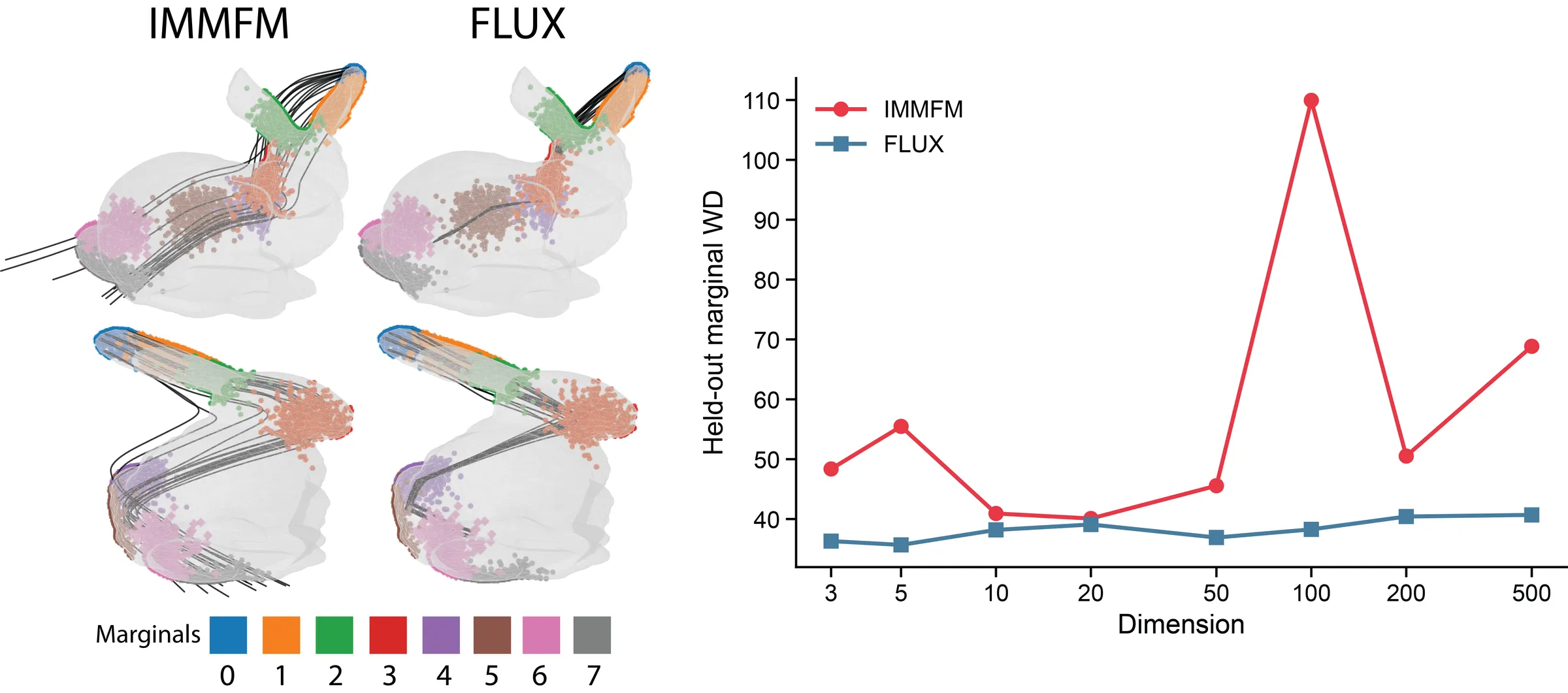
A geodesic path on a known 3D mesh, embedded in ambient dimensions up to 100, with two marginals held out. Tests whether transport stays on the manifold.
Longitudinal Flow Matching with Mixture of Experts
Yale University
TL;DR. Many biological processes are observed only as unpaired snapshots at successive stages. FLUX learns one velocity field that transports these snapshots along geometry-aware paths on the data manifold, and splits it into sparse expert vector fields, so the router’s choice of expert becomes an unsupervised label for when the dynamics change.
Many biological systems evolve through continuous local dynamics while switching between latent regimes defined by learning, stimulus context, internal state, or developmental stage. These processes are often observed only as unpaired longitudinal snapshots: the same cells, neurons, or animals are not tracked as matched trajectories, even though population states are sampled across successive stages. Two coupled challenges follow. Trajectories must respect curved low-dimensional manifolds embedded in high-dimensional measurements, and the model must identify when the transport mechanism itself changes.
FLUX (Flow matching for Unpaired longitudinal data with miXture-of-experts) learns a data-dependent metric from pooled labeled and unlabeled observations, uses it to construct geometry-aware conditional paths between adjacent marginals, and decomposes the resulting velocity field into sparse expert vector fields selected by a Straight-Through Gumbel-Softmax router.
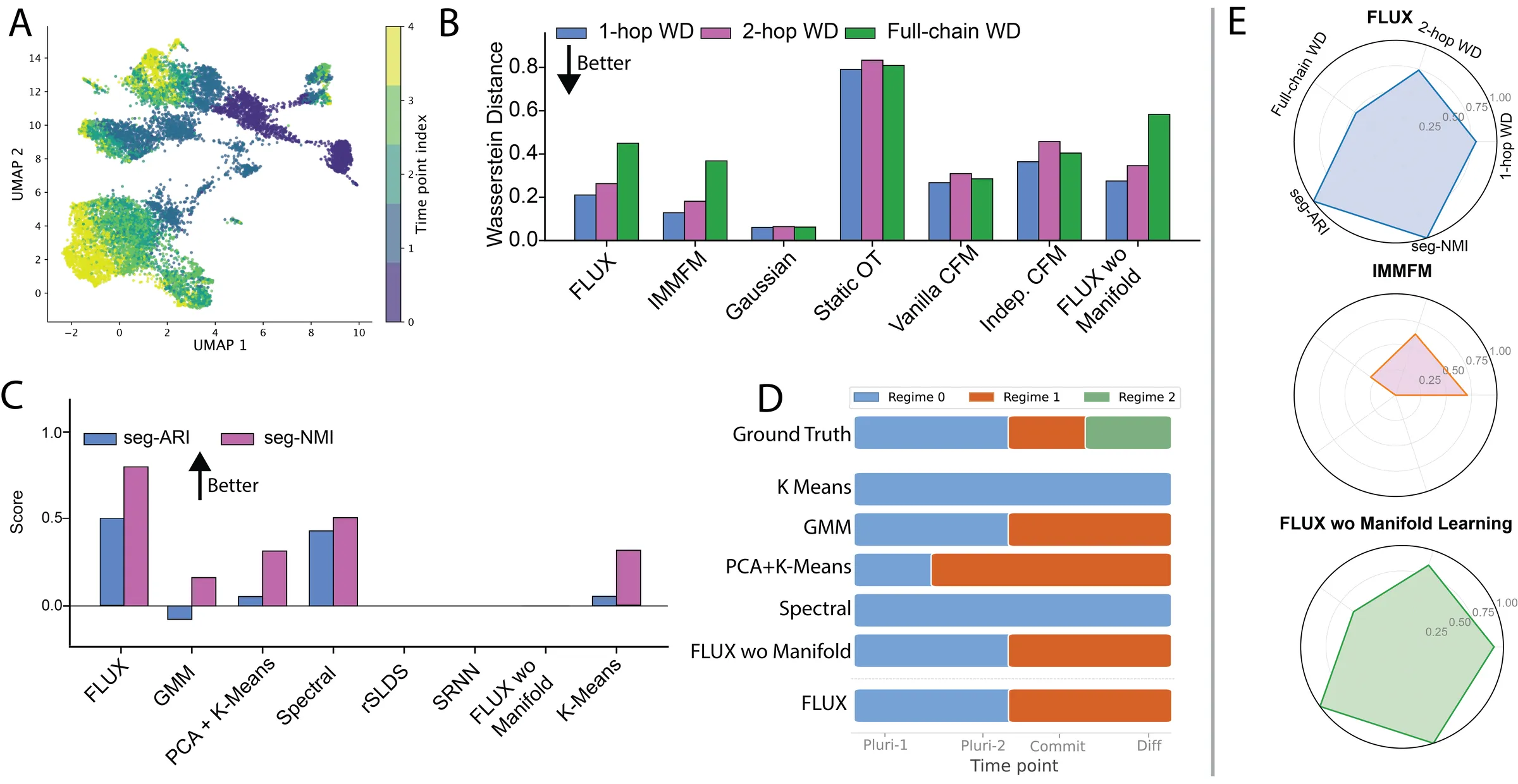
Across manifold controls, a regime-switching Lorenz system, widefield cortical calcium imaging during associative learning, and embryoid-body single-cell differentiation, FLUX reconstructs longitudinal transport while recovering interpretable regime structure. Ablations show that mixture-of-experts routing alone is not enough: without geometric learning, FLUX can fit local transport but fails or weakens at regime discovery when regimes are encoded in local dynamics.
One velocity field trained on adjacent pairs of unpaired snapshots, integrated across the whole chain.
A learned metric and bend network keep interpolants on the data manifold instead of crossing empty space.
A mixture of expert vector fields; the hard routing decision is an unsupervised regime label.
Training has three stages. A metric is learned from pooled observations, a bend network turns straight interpolants into geometry-aware paths, and a mixture-of-experts velocity field is trained on those paths. The geometry and bend networks are frozen before velocity training.
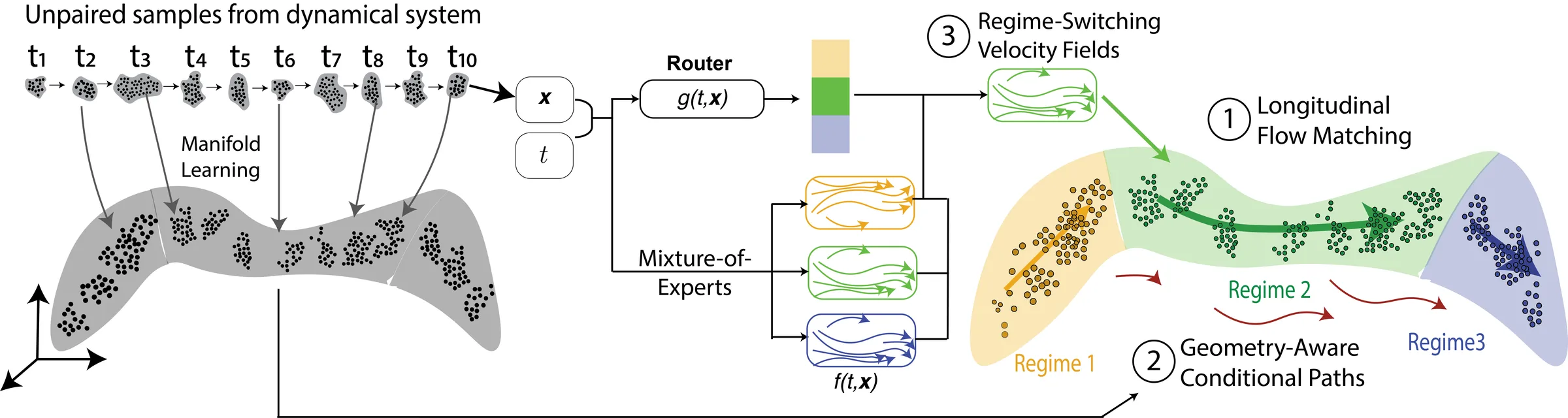
Observations arrive as \(T\) ordered marginals \(\mu_1,\dots,\mu_T\) with no correspondence between samples. For each adjacent pair \((\mu_k, \mu_{k+1})\), FLUX draws endpoints from a coupling \(\pi_k\), samples a local time \(\tau\), and maps it to a global model time.
Every pair supervises the same velocity field, so its ODE can be integrated from the first snapshot to the last.
Straight interpolation between endpoints can pass through low-density regions when data concentrate near a curved manifold. FLUX learns a manifold score \(h_\theta\) from pooled observations, including unlabeled samples, and turns it into a metric that is cheap on the data and expensive off it.
A bend network \(\Delta_\psi\) then displaces the straight interpolant; the resulting path supplies both the training locations and the velocity targets. The metric reshapes supervision and is not an input to the velocity network.
The velocity field is a mixture of \(M\) expert vector fields. A router maps each (time, state) pair to logits, and Straight-Through Gumbel-Softmax makes the assignment near-discrete in the forward pass while keeping gradients. The Gumbel temperature is annealed from 1.0 to 0.05–0.2.
At inference the hard assignment is an unsupervised regime label: a decomposition of the learned transport rather than a clustering of static snapshots. Router regularizers encourage sparse, temporally coherent assignments and prevent expert collapse.
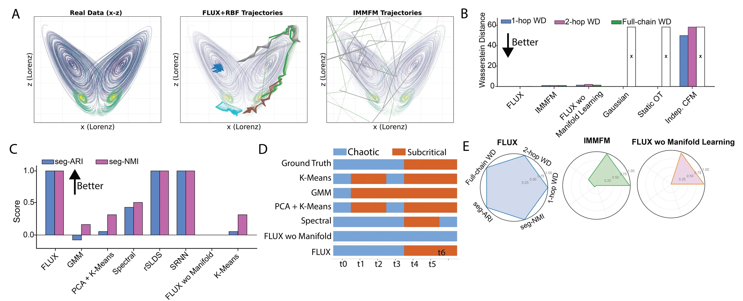
FLUX recovers known regime switches without labels and keeps transport on the data manifold as ambient dimension grows. Behavioral and stage labels are used only for evaluation.
Lorenz segment ARI / NMI: FLUX recovers the chaotic-to-subcritical switch exactly (IMMFM: 0.05 / 0.32)
Segment NMI on embryoid-body differentiation (pluripotent, commitment, differentiated)
Highest ambient embedding of the Stanford Bunny manifold control
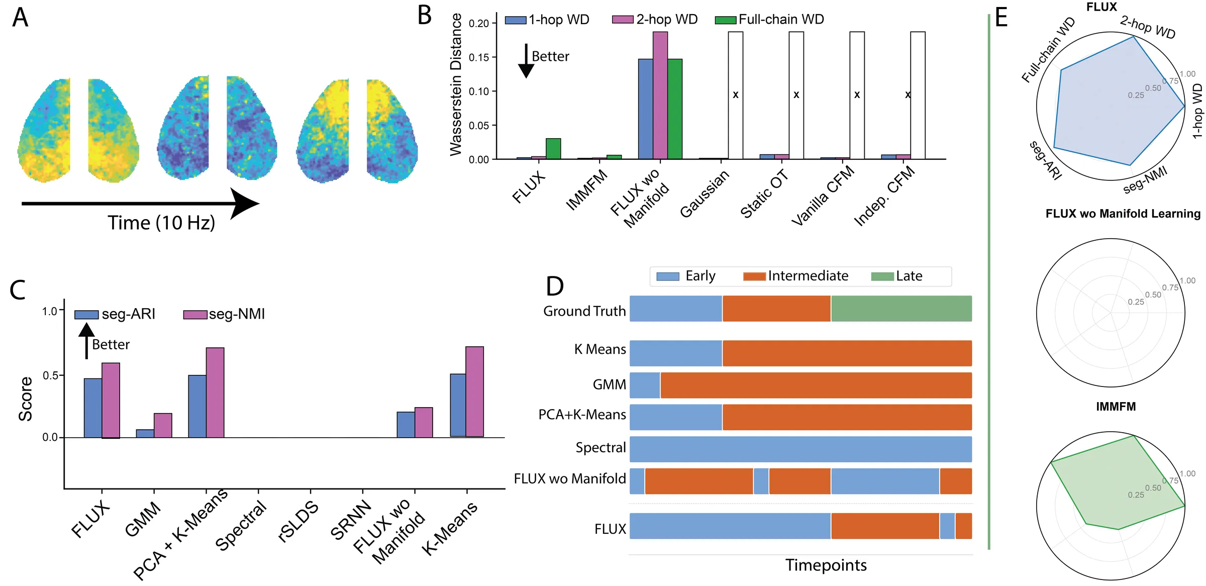
Widefield calcium imaging: 41 cortical areas over 22 days of learning
Manifold control
8 marginals · up to 100-D
A geodesic path on a known 3D mesh, embedded in ambient dimensions up to 100, with two marginals held out. Tests whether transport stays on the manifold.
Dynamical system
8 marginals · 60-D
Chaotic versus lower-ρ regimes from flattened 3 × 20 trajectory windows, with a known dynamical transition between marginals 3 and 4.
Neuroscience
22 day marginals · 451-D
12 mice, 41 cortical areas, Go/No-Go visual associative learning. Behavioral labels are used only for evaluation, never for training or routing.
Single-cell biology
5 time points · scRNA-seq
Up to 1,000 cells per marginal in PCA space. Pluripotent, commitment, and differentiated stage labels are withheld during training.
Code release coming soon. The commands below preview the pipeline on the Lorenz benchmark; each stage writes a checkpoint that the next stage loads. Evaluation uses compute_metrics.py.
Fit the RBF manifold score (or a VAE-based geometry) for the benchmark. Output: rbf_network_best.pth.
python scripts/benchmark_data/train_benchmark_rbf.py \
  --dataset lorenz --lorenz_mode day_marginals --num_marginals 8 \
--save_dir saved_models/lorenzLearn geometry-aware conditional paths using the frozen metric. Output: bend_network_best.pth.
python scripts/benchmark_data/train_benchmark_bend.py \
  --dataset lorenz --lorenz_mode day_marginals --num_marginals 8 \
  --geo_model_path saved_models/lorenz/rbf_network_best.pth \
  --save_dir saved_models/lorenz
Train the velocity field with Gumbel routing on the frozen paths. Output: velocity_network_best.pth.
python scripts/benchmark_data/train_benchmark_velocity.py \
  --dataset lorenz --lorenz_mode day_marginals --num_marginals 8 \
  --geo_model_path saved_models/lorenz/rbf_network_best.pth \
  --bend_model_path saved_models/lorenz/bend_network_best.pth \
  --use_gumbel_routing --num_experts 2 --save_dir saved_models/lorenz

python scripts/benchmark_data/compute_metrics.py \
--dataset lorenz --model_dir saved_models/lorenzIf you use FLUX in your research, please cite:
@inproceedings{ortegacaro2026flux,
  title     = {{FLUX}: Longitudinal Flow Matching with Mixture of Experts},
  author    = {Ortega Caro, Josu{\'e} and Zhang, Yongxu and Batchelor, Hannah M.
               and He, Sizhuang and Cardin, Jessica A. and Saxena, Shreya},
  booktitle = {Advances in Neural Information Processing Systems (NeurIPS)},
  year      = {2026},
  eprint    = {2605.08648},
  archivePrefix = {arXiv}
}