FLUX

Geometry-Aware Longitudinal Flow Matching with Mixture of Experts

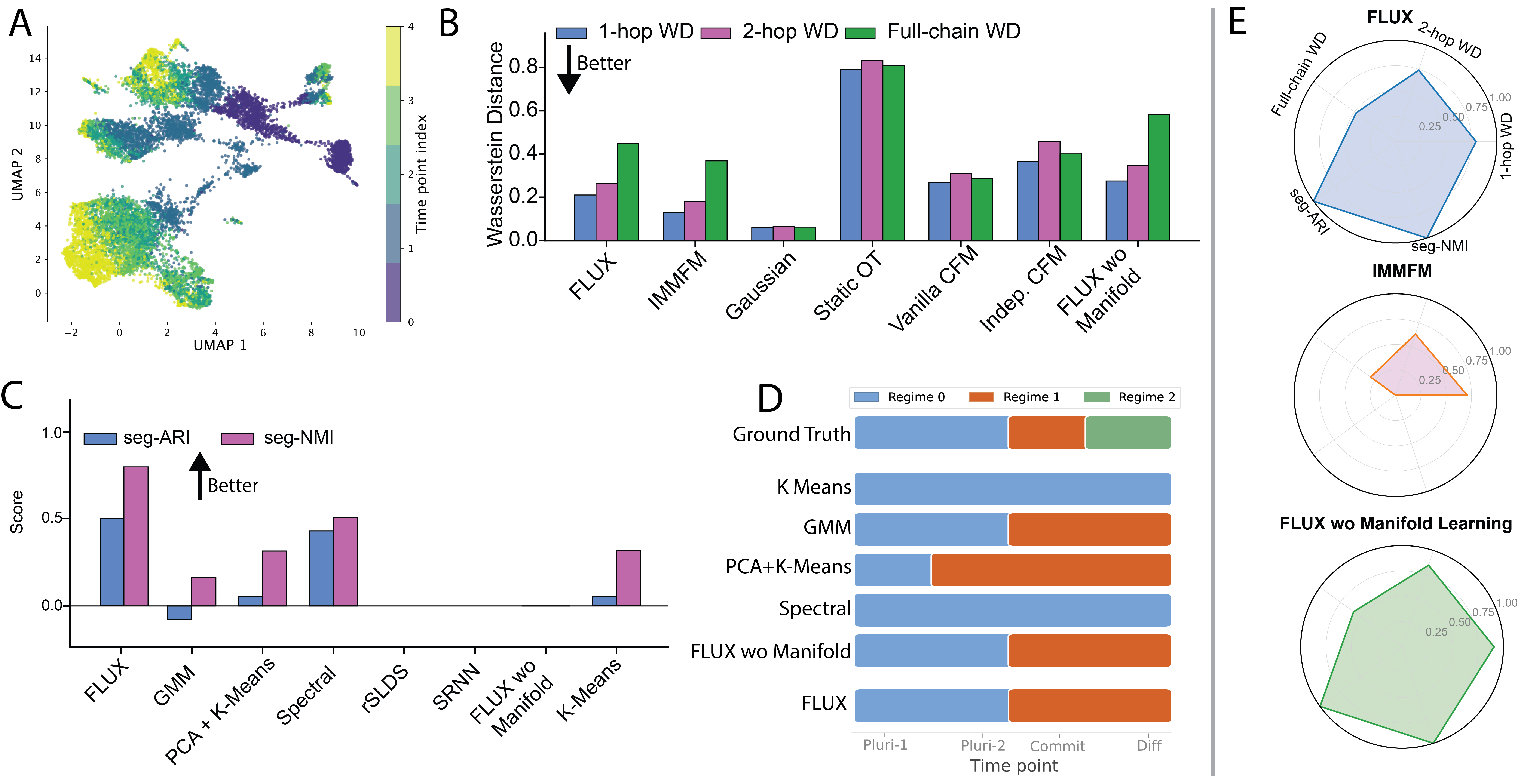
Many biological systems evolve through continuous dynamics while switching between latent regimes, yet are observed only as unpaired longitudinal snapshots. FLUX learns a data-dependent geometry to construct manifold-aware conditional paths between adjacent marginals and decomposes the resulting velocity field into sparse expert vector fields for joint transport modeling and unsupervised regime discovery.

Josue Ortega Caro Yongxu Zhang Hanna M. Batchelor Sizhuang He Jessica Cardin Shreya Saxena

Yale University · Wu Tsai Institute · Kavli Institute

Overview of FLUX: unpaired marginal snapshots, geometry-aware conditional paths via a learned metric and bend network, and a mixture-of-experts velocity field with Gumbel-Softmax routing.
Longitudinal data are observed as unpaired population snapshots. FLUX uses learned geometry for manifold-aware conditional paths across ordered marginals, and a regime-switching velocity field with Straight-Through Gumbel-Softmax routing.
Abstract Method Results Benchmarks Pipeline Usage Cite

Joint transport modeling and regime discovery

Many biological systems evolve through continuous local dynamics while switching between latent regimes defined by learning, stimulus context, internal state, or developmental stage. These processes are often observed only as unpaired longitudinal snapshots: the same cells, neurons, or animals are not tracked as matched trajectories, even though population states are sampled across successive stages. This creates two coupled challenges. First, trajectories must respect curved low-dimensional manifolds embedded in high-dimensional biological measurements. Second, the model must identify when the transport mechanism itself changes.

We introduce FLUX (Flow matching for Unpaired longitudinal data with miXture-of-experts), a geometry-aware longitudinal flow-matching framework for joint transport modeling and unsupervised regime discovery. FLUX learns a data-dependent metric from pooled labeled and unlabeled observations, uses that metric to construct geometry-aware conditional paths between adjacent marginals, and decomposes the resulting velocity field into sparse expert vector fields selected by a Straight-Through Gumbel-Softmax router.

Across manifold controls, a regime-switching Lorenz system, widefield cortical calcium imaging during associative learning, and embryoid body single-cell differentiation, FLUX reconstructs longitudinal transport while recovering interpretable regime structure. Ablations show that mixture-of-experts routing alone is insufficient: FLUX without geometric learning can fit local transport but fails or weakens regime discovery when regimes are encoded in local dynamics. These results suggest that geometry-aware velocity decomposition provides a general strategy for discovering latent biological state transitions from unpaired longitudinal snapshots.

How FLUX works

FLUX combines three ideas: longitudinal marginal chaining, geometry-aware conditional paths, and a mixture-of-experts velocity field.

Adjacent-marginal chaining

FLUX observes T ordered marginal distributions at discrete observation times. Each marginal contains unpaired samples—consecutive snapshots do not correspond to the same cell, neuron, or individual. FLUX trains on adjacent marginal pairs: for each pair, endpoints are sampled from an optimal-transport coupling, a local interpolation time is drawn, and the resulting point and tangent are mapped to global model time. This yields a single velocity field whose ODE is integrated across the full marginal chain.

From Euclidean shortcuts to manifold-aware paths

Standard flow matching uses Euclidean linear interpolation between endpoints, which can pass through low-density regions when data concentrate near a curved manifold. FLUX instead learns a data-dependent metric G from pooled observations (including unlabeled samples when available), then trains a bend network B that parameterizes approximate geodesic paths. The geometry-aware path replaces the Euclidean interpolant everywhere: it changes the training locations, the target tangents, and where the velocity network is evaluated. The metric is not an input to the velocity network—it reshapes the conditional paths used for supervision.

Sparse expert routing for regime discovery

FLUX decomposes the velocity field into M expert vector fields. A router maps each (time, state) pair to expert logits, and Straight-Through Gumbel-Softmax produces differentiable but near-discrete routing weights during training. At inference, the hard expert assignment provides an unsupervised candidate regime label—a decomposition of the learned transport dynamics rather than post-hoc clustering of static observations. Router regularizers encourage sparse, temporally coherent assignments and discourage expert collapse.

Experiments

Stanford Bunny dimensionality ablation: eight ordered marginals on a geodesic path, held-out Wasserstein distance across ambient dimensions 3 to 100.
Stanford Bunny dimensionality ablation. Eight ordered marginals are sampled on a geodesic path over the Stanford Bunny mesh, with two intermediate marginals held out from velocity training. The same surface is embedded into higher-dimensional spaces (D = 3, 5, 10, 20, 50, 100). Geometry-aware paths preserve surface transport and interpolate to unseen marginals, while Euclidean baselines cut through the mesh interior as ambient dimension increases.
Lorenz dynamical-system benchmark: transport metrics, regime-discovery metrics, temporal regime assignments, and radar summary.
Lorenz dynamical-system benchmark. (A) Two-dimensional visualization of trajectory-window samples colored by the ground-truth Lorenz parameter regime. (B) Generative transport metrics. (C) Segment-level regime-discovery metrics (ARI and NMI). (D) Temporal regime assignments predicted by each method compared with the ground-truth parameter switch. (E) Radar summary. FLUX recovers the chaotic/subcritical boundary exactly (seg-ARI = 1.0, seg-NMI = 1.0), while FLUX without manifold learning collapses to a single expert.
Widefield calcium-imaging benchmark: cortical activity, transport metrics, regime-discovery metrics, temporal expert assignments, and radar summary.
Widefield calcium-imaging benchmark. (A) Example post-stimulus cortical activity represented as brain area by time, flattened into a 451-dimensional vector. (B) Generative transport metrics. (C) Segment-level regime-discovery metrics. (D) Temporal expert assignments compared with early, intermediate, and late behavioral learning labels. (E) Radar summary. The router separates early/intermediate from late training, coinciding with the behavioral divergence of CS+ and CS− lick indices.
Embryoid body differentiation benchmark: UMAP projections colored by differentiation stage, transport metrics, regime-discovery metrics, temporal expert assignments, and radar summary.
Embryoid body differentiation benchmark. (A) RNA-seq profiles projected into UMAP space and colored by differentiation stage. (B) Generative transport metrics. (C) Segment-level regime-discovery metrics. (D) Temporal expert assignments compared with pluripotent, commitment, and differentiated stage labels. (E) Radar summary. FLUX separates expression-evolution regimes associated with pluripotent and more differentiated cell populations.

Datasets

Stanford Bunny
8 marginals
Geodesic path on a known 3D mesh, embedded into ambient dimensions up to 100. Two marginals held out for evaluation. Tests whether geometry-aware transport stays on the manifold.
Lorenz
8 marginals · 60-D
Chaotic vs lower-ρ regimes from flattened 3×20 trajectory windows. Known dynamical transition between marginals 3 and 4.
Widefield Ca2+
22 day marginals · 451-D
12 mice, 41 cortical areas, Go/No-Go visual associative learning. Behavioral labels used for evaluation only, not during training or routing.
Embryoid body (EB)
5 timepoints · scRNA-seq
Up to 1,000 cells per marginal in PCA space. Pluripotent, commitment, and differentiated stage labels withheld during training.

Three-stage training

Geometry and bend networks are frozen before velocity training. Evaluation uses compute_metrics.py.

Stage Script Output
1. Geometry train_benchmark_rbf.py or train_benchmark_vae.py rbf_network_best.pth or best_gaga_model.pth
2. Bend train_benchmark_bend.py bend_network_best.pth
3. Velocity train_benchmark_velocity.py velocity_network_best.pth

Install and run (Lorenz)

See the repository README for full options, conda setup, and dataset-specific flags.

Clone and environment

git clone https://github.com/josueortc/flux.git
cd flux
conda create -n flux python=3.10 -y && conda activate flux
# Install PyTorch for your platform, then:
pip install -r requirements.txt
1

Metric (RBF)

Learn the Riemannian metric for your benchmark dataset.

python scripts/benchmark_data/train_benchmark_rbf.py \
  --dataset lorenz --lorenz_mode day_marginals --num_marginals 8 \
  --save_dir saved_models/lorenz
2

Bend network

Train the bend network using the saved geometry checkpoint.

python scripts/benchmark_data/train_benchmark_bend.py \
  --dataset lorenz --lorenz_mode day_marginals --num_marginals 8 \
  --geo_model_path saved_models/lorenz/rbf_network_best.pth \
  --save_dir saved_models/lorenz
3

Velocity + MoE

Train the mixture-of-experts velocity with Gumbel routing, then evaluate.

python scripts/benchmark_data/train_benchmark_velocity.py \
  --dataset lorenz --lorenz_mode day_marginals --num_marginals 8 \
  --geo_model_path saved_models/lorenz/rbf_network_best.pth \
  --bend_model_path saved_models/lorenz/bend_network_best.pth \
  --use_gumbel_routing --num_experts 2 --save_dir saved_models/lorenz

python scripts/benchmark_data/compute_metrics.py \
  --dataset lorenz --model_dir saved_models/lorenz

Citation

If you use FLUX in your research, please cite:

@article{ortegacaro2026flux,
  title={FLUX: Geometry-Aware Longitudinal Flow Matching with Mixture of Experts},
  author={Ortega Caro, Josue and Zhang, Yongxu and Batchelor, Hannah M. and He, Sizhuang and Cardin, Jessica and Saxena, Shreya},
  journal={arXiv preprint arXiv:2605.08648},
  year={2026}
}