Preprint · bioRxiv 2025

PRISMt

Pattern Reconstruction and Interpretation of Structured Motifs in transformers

Josué Ortega Caro Hannah M. Batchelor Sweyta Lohani David van Dijk Jessica A. Cardin

Department of Neuroscience · Kavli Institute for Neuroscience · Wu Tsai Institute · Yale University

TL;DR. Transformers can model neural recordings across regions, time, and modalities, but standard attribution collapses those axes into one importance map. PRISMt maps a transformer’s classification-token attribution back onto the native axes of the recording and decomposes it into spatial, temporal, and modality-resolved motifs that are faithful to what the model actually uses. In cortical calcium and acetylcholine imaging during learning, it revealed cholinergic motifs reorganizing toward frontal cortex.

ΔF/F (low → high) masked token future (not attended)
Illustrative The 41-region cortical grid used in the paper, one map per modality, with synthetic responses. Every region, time bin, and modality becomes a token; a query token (circled) attends only to the present and past, and masked tokens are reconstructed from that causal context. Switch to late learning to see acetylcholine responses shift from posterior visual toward frontal cortex, the kind of change PRISMt resolved in real data.
Overview

Interpreting transformers of multidimensional neural data

Large-scale recordings increasingly combine signals across brain regions, time, and measurement modalities. Transformers can relate all of these in parallel, but interpreting them is a separate problem. Attention rollout describes how information is routed through the layers, and gradient- or relevance-based methods add class sensitivity, yet both characterize model tokens rather than the experimentally meaningful axes of the recording. Decomposing the observations alone finds dominant structure in the data, not the structure used for a particular prediction.

PRISMt is applied to a trained classification-token transformer. It combines attention-mediated routing with the signed value message carried by each token, maps the result back onto sample, region, time, and modality, reduces it across layers and heads, and factorizes it into structured motifs that can be aligned across model fits and experimental conditions. Masked autoencoding learns distributed neural structure; PRISMt identifies the structured signals that drive a specific prediction.

Attribution on the recording’s axes

Region × time × modality, per trial, instead of one collapsed importance map.

Structured motifs

Non-negative CP factors with separate spatial, temporal, and modality profiles, comparable across conditions.

Faithful to the model

Distinguishes pathways the classifier uses from correlated decoys present in the data.

Method

How PRISMt works

A multimodal transformer is pretrained by masked autoencoding under block-causal attention and fine-tuned with a CLS token. PRISMt then turns each prediction into a region × time × modality attribution tensor and decomposes it into motifs.

1

One token per region, time, and modality

Each trial is a tensor \(X_n \in \mathbb{R}^{R\times T\times M}\). Every scalar observation becomes a token: it is projected to the model dimension (\(d = 512\)) and combined with a learned token embedding. For the cortical dataset, \(R = 41\) regions, \(T = 10\) time bins, and \(M = 2\) modalities give 820 data tokens per trial.

A learned CLS token provides the sequence-level representation used for classification.

Token embedding\[ z^{(0)}_{n,i} = W_E\, x_{nrtm} + b_E + p_i, \qquad i = \tau(r,t,m) \]
Illustrative A toy trial with 4 regions, 5 time bins, and 2 modalities. Tokens are ordered by time: all regions and modalities at the first bin, then the next.
2

Learn distributed structure by masked autoencoding

During pretraining, 90% of data tokens are replaced by a learned mask embedding and the model reconstructs them from the remaining context. The loss is evaluated only on masked tokens.

Try it: mask cells, then reconstruct. The estimate here is a toy that uses the information available under block-causal attention: the past of each region and other tokens at the same time.

Masked reconstruction loss\[ \mathcal{L}_{\mathrm{MAE}} = \frac{1}{\sum_n |\Omega_n|} \sum_n \sum_{i\in\Omega_n} \big\lVert \hat z_{n,i} - z^{(0)}_{n,i} \big\rVert_2^2 \]
Illustrative Synthetic traveling-wave signal. Reconstructed cells are outlined and filled bin by bin, because each estimate may use only the current and earlier time bins. This toy estimator is not the trained model.
3

Block-causal attention

A token at time \(t\) attends to all regions and modalities at the same time and to every token at earlier times, never to future bins. The same backbone models recordings whose modalities differ in scale, noise, and temporal structure.

Attention with the block-causal mask\[ A^{(\ell,h)}_{n,ij} = \operatorname{softmax}_j\!\left( \frac{q_{n,i}^{\top} k_{n,j}}{\sqrt{d_h}} + M_{ij} \right), \qquad M_{ij} = \begin{cases} 0 & t_j \le t_i \\ -\infty & t_j > t_i \end{cases} \]
Filled cells are allowed query → key pairs. Hover a cell to highlight its row and column.
4

Attribute the prediction to region, time, and modality

For every layer \(\ell\), head \(h\), and token, PRISMt multiplies the residual-aware rollout coefficient \(\rho\) (how much the token is routed to CLS) by the token’s signed value message projected onto the direction of the target logit \(\zeta_n\).

Layer–head pairs are then weighted by how strongly their attribution differs between classes, removing the transformer-specific axes while keeping sample, region, time, and modality.

Token attribution\[ G_n^{(\ell,h)}(r,t,m) = \rho^{(\ell,h)}_{n,i}\; u_n^{\top} W_O^{(\ell,h)} v^{(\ell,h)}_{n,i}, \qquad u_n = \frac{\nabla_{h_{n,\mathrm{CLS}}}\zeta_n}{\lVert \nabla_{h_{n,\mathrm{CLS}}}\zeta_n \rVert_2} \]
Layer–head reduction\[ w_{\ell h} = \frac{D_{\ell h}}{\sum_{\ell',h'} D_{\ell' h'}}, \qquad \tilde G_n(r,t,m) = \sum_{\ell,h} w_{\ell h}\, G_n^{(\ell,h)}(r,t,m) \]
Illustrative Synthetic example with a used pathway (frontal ACh, late bins) and a correlated decoy (visual calcium, early bins). Routing alone lights up both; combining routing with signed messages and discriminative layer–head weights keeps the pathway the classifier uses.
5

Decompose into structured motifs

PRISMt factorizes the magnitude of the reduced attribution tensor with a non-negative canonical polyadic decomposition. Each motif has a sample factor \(a_k(n)\), a spatial profile \(d_k(r)\), a temporal profile \(e_k(t)\), and a modality allocation \(f_k(m)\) constrained to the simplex, so every motif sits on a common modality scale.

Motifs are calcium- or ACh-dominant when one modality weight exceeds 0.65 and shared otherwise, and they are aligned across cross-validated fits and bootstrap resamples before conditions are compared.

Motif decomposition\[ T_n(r,t,m) \approx \sum_{k=1}^{K} \lambda_k\, a_k(n)\, d_k(r)\, e_k(t)\, f_k(m), \qquad f_k(m) \ge 0,\;\; \sum_m f_k(m) = 1 \]
Illustrative Three motifs with spatial, temporal, and modality factors on the 41-region grid. Across learning, the calcium-dominant motif stays broadly distributed while the ACh-dominant motif shifts from posterior visual toward frontal cortex, as PRISMt found in the imaging data.
Benchmarks

Recovery and faithfulness on synthetic systems

All synthetic systems come from the same 64-unit recurrent network trained on a NeuroGym two-alternative perceptual decision task, projected to 32 regions and two modalities, so they differ only in how task-relevant information is arranged. Recovery asks whether a method finds the pathways placed in the data; faithfulness asks whether attribution follows the pathways the classifier uses.

0.987

Unit-support AUROC, System 1 (one modality-specific pathway)

0.975

System 2 (two separated modality-specific pathways)

0.795

System 3 (adds a shared pathway with gain increasing across trials)

0.937

Decoy system, primary pathway (observation-level methods: 0.547–0.827)

The decoy test

Correlated is not the same as used

In System 4 a decoy pathway is correlated with held-out labels but never learned by the classifier. Observation-level decompositions recover both pathways; PRISMt places essentially no attribution on the decoy (causal allocation agreement 1.000, false-attribution mass 0.000).

Operating range

14 of 20 decoy configurations

Across a sweep of decoy informativeness and pathway gain, PRISMt outperformed the observation-level baseline in 14 of 20 settings; most failures occurred where occlusion showed the classifier had switched to the decoy.

Generalization

Different multimodal recordings

The same backbone modeled spontaneous activity in dual-color calcium/ACh3.0 imaging and in mesoscale calcium imaging combined with extracellular electrophysiology, exceeding a channel-mean floor in both.

Application

Cortical calcium and acetylcholine during learning

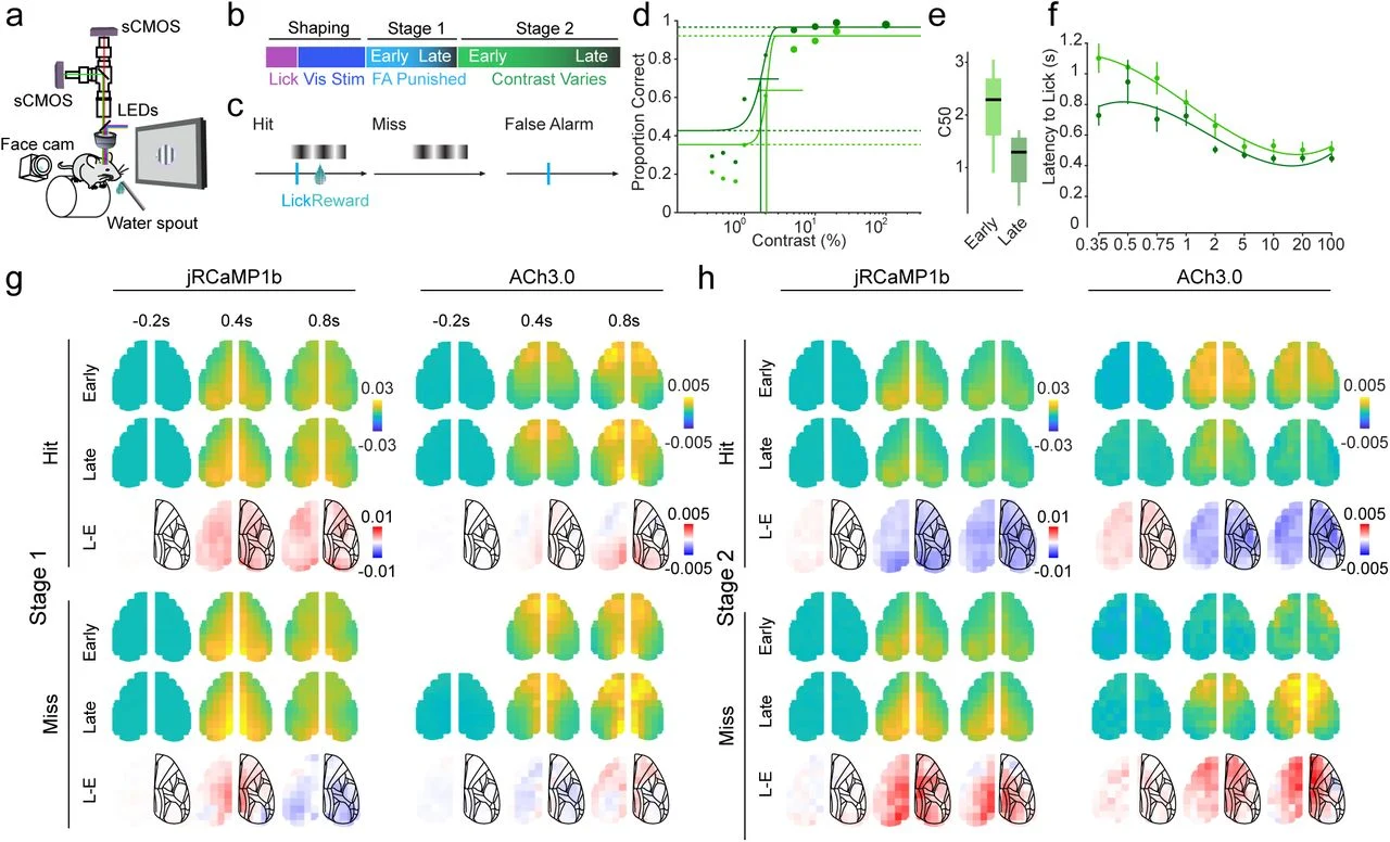
Mice expressing the calcium indicator jRCaMP1b and the acetylcholine sensor GRAB-ACh3.0 throughout cortex were imaged through the intact skull while learning a visual detection task, first response timing (Stage 1) and then contrast detection (Stage 2).

The transformer reconstructed masked signals, predicted forward in time, and generalized to held-out mice; behavioral prediction was strongest when calcium and ACh3.0 were modeled together. Applying PRISMt to these models, calcium-associated motifs remained broadly distributed across frontal, somatosensory, and visual cortex, whereas ACh-associated motifs shifted from posterior visual cortex toward frontal cortex across Stage 2 learning, consistently across individual mice.

Two independent objectives agreed: ACh3.0 became more predictable in anterior cortex under both random masking and forward prediction, while jRCaMP1b changed little. Regions selected by PRISMt also became more strongly coordinated in the cholinergic signal after learning.

Calcium

Distributed motifs; little learning-related change in predictability.

Acetylcholine

Motifs reorganize toward frontal subnetworks; anterior predictability and connectivity increase.

Dual-color mesoscopic imaging setup, task stages, trial outcomes, behavioral performance across learning, and cortex-wide jRCaMP1b calcium and ACh3.0 acetylcholine maps for hit and miss trials early and late in learning.
Dual-color imaging across learning (from the bioRxiv preprint). (a) Mesoscopic imaging setup. (b) Task stages. (c) Trial outcomes. (d–f) Behavioral performance across learning. (g, h) Cortex-wide calcium (jRCaMP1b) and acetylcholine (ACh3.0) maps for hit and miss trials, early and late in learning, and their difference (L − E).
Architecture

Predictive backbone and interpretation

The model and its interpretation are separate: the transformer learns to predict; PRISMt explains the prediction.

InputR × T × M TokenizeLinear(1 → 512)+ token embedding+ CLS token Mask90% of tokenslearned [MASK] Decoder-only Transformerblock-causal attentionresidual + layer normtwo-layer feedforward× L layers Reconstructionloss on masked tokens CLS headbehavioral classification AdamW · batch 128 · lr 5×10⁻⁴ with cosine annealing · ≤ 200 epochs, early stopping
Usage

Getting started

See the repository for installation and the current command-line options.

Prepare your data

Organize each trial as regions × time × modality in the standardized .mat format, using the MATLAB scripts or the GUI.

% In MATLAB
run_prismt_gui   % launch the GUI
% or:
standardize_data('your_data.mat', 'output_standardized.mat')

Pretrain and fine-tune the transformer

python train.py --data_path data/standardized.mat --task_name phase_classification

Run PRISMt attribution and motif analysis

python analyze_results.py \
  --checkpoint results/best_model.pt \
  --data_path data/standardized.mat \
  --output_dir results/analysis/

Configuration used in the paper

tokens (cortex)41 × 10 × 2 + CLS
model dim d512
mask ratio90%
optimizerAdamW
weight decay1e-2
batch size128
learning rate5e-4, cosine
epochs≤ 200
early stoppingpatience 20
grad clip1.0
CP restarts5 × 2,000 iter
modality threshold0.65
Citation

Cite this work

If you find PRISMt useful, please cite the preprint:

@article{ortegacaro2025cholinergic,
  title     = {Selective changes in cortical cholinergic signaling during learning},
  author    = {Ortega Caro, Josu{\'e} and Batchelor, Hannah M. and Lohani, Sweyta
               and van Dijk, David and Cardin, Jessica A.},
  journal   = {bioRxiv},
  year      = {2025},
  doi       = {10.1101/2025.08.29.673096},
  publisher = {Cold Spring Harbor Laboratory}
}