Using Q-Learning in Numpy to teach an agent to play a game

10 minute read

There are some Machine Learning models which can be trained to map any given input to a desired output based on the input-output pair used during training. By input-output pair, I obviously mean the input and it’s respective ground truth or labels. Such algorithms are called Supervised Learning algorithms. Classification and Regression are some of it’s examples.

Also, there exists a class of machine learning models that look for underlying patterns in the data, without requiring the knowledge of the labels explicitly. These algorithms are called Unsupervised Learning algorithms. Clustering and Density Estimation are some of it’s examples.

Then there is this third kind of machine learning paradigm, alongside supervised learning and unsupervised learning, called the Reinforcement Learning which is fundamentally different from the prior two types.

This basically involves making sequential decisions in an environment in order to maximize the cumulative future rewards. I will explain this in greater detail in a while.

Q-Learning is one such model-free Reinforcement Learning algorithm that learns to make correct actions under various circumstances.

Let us first get familiar with the very basic terminologies of a Reinforcement Learning set-up.

Let’s get familiar with some basic RL terminologies

There is something called an environment that literally consists of everything that the system is made up of. It has an agent that observes the environment (takes inputs from the environment) and then takes actions based on the inputs, changing the state of the environment and collecting rewards in the process.

Do not worry if this does not make perfect sense to you yet !

Let us try to understand this with the help of an example.

So there is a 6x6grid. We have our agent randomly spawned at one of the 6x6=36 possible cells in the grid. Similarly we have a bottle of beer and a deadly virus at two other cells in our grid world. The agent, the bottle of beer and the deadly virus will spawn at unique cell positions every time. The agent wants to reach to the bottle of beer avoiding the virus which might infect it and therefore end the game. The restriction on agent’s movement is that it can only move one cell in any diagonal direction.

In this set-up, our 6x6 grid-world is the environment. The agent has access to it’s relative position with respect to the bottle of beer (reward) and the deadly virus (enemy), and we call this information about the environment that the agent has access to, as state. And the agent can take certain predefined actions, like moving a cell in any of the four diagonal directions, depending on the current state of the environment. Agent’s action might get it a bottle of beer (a positive reward) or it might get the agent infected by the deadly virus (a negative reward). So the objective of the agent here is to learn about it’s environment by interacting with it and ultimately learn to take actions such that the future cumulative sum of rewards gets maximized.

The sequence of states, actions and rewards until it all ends (either by reaching to the beer bottle or getting infected by the virus), is called an episode.

The states which cause the episode to terminate are called the terminal states. In our example of the grid-world, the states in which the relative position of the agent either with respect to the beer bottle or the virus, becomes zero, are the terminal states.

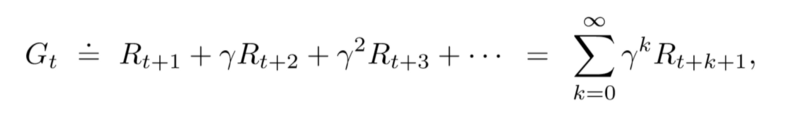
Return is the cumulative sum of the future rewards. This might reach infinity in cases where there are no terminal states, also known as Non-Episodic tasks. To make it a finite sum, we discount the future rewards using a discounting factor called gamma.

Following is the formula for return at time t, expressed in terms of rewards at various time steps. Here T is the final time step and Γ is the discount rate such that 0 ≤ Γ ≤ 1

Value function are the functions of the states (or the state-action pairs) that estimate how good it is for the agent to be in a given state (or how good is it to perform a given action in a given state)

Value functions are always defined with respect to particular ways of acting, called policies.

A policy is nothing but a mapping from states to probabilities of selecting each possible action.

I would like to talk more about the state-action value function because we are going to make use of it in the rest of the blog.

So as mentioned earlier, a state-action function is a function that returns the expected return starting from a state ‘s’, taking action ‘a’ and thereafter following the policy π.

So comparing the values of a state-action function for a given state and all the actions in the action space, can lead us to the best possible action that can be taken in that state. And this is actually how our agent is going to choose the best action that can be taken in a given state.

Q-Table is a table consisting of all the state-action pairs. It’s like a look-up table from where, if give a current state and action, we can get the state-action or the q-value.

We initialize the q-table with random numbers initially and then keep on updating the vales for each state-action pair as the agent continues to take various actions under various states. After a certain degree of exploration of the environment by the agent, we can, by using the q-table tell which would be the best action to be taken for any given state !

Isn’t that crazy ! :D

Let’s get our hands dirty !

We are going to learn how to implement q-learning now. This is going to be a fun ride. Fasten your seat belts :D

We start by importing all the necessary libraries.

Then we define all the hyperparameters of the q-learning algorithm and the display window.

Next we define the path of the images for our agent, beer bottle (positive reward) and the virus (negative reward) and read them to be displayed on the screen. This is just to make the display window look interesting.

We need to make a class called ‘Blob’ which our agent, beer bottle and the virus would inherit. A Blob class object would have a spawning location (x and y coordinates) associated with it and it would be able to move diagonally depending on the input passed in it’s ‘move’ method. We would also be able to add to subtract two Blob objects. It would simple add or subtract the x and y coordinates of the two Blob objects.

Let’s define the q-table now, which will be used again and again to pick the best action under a given state. And we will constantly keep on updating this table to improve the decision making ability of our agent.

Note that the range here that we have taking for the state-space is -SIZE+1 to SIZE. This is because we have defined the state-space as the relative position of the agent from the beer bottle and the virus. So this can be positive or negative. For exmaple, if the SIZE of the grid-world is 6, then the relative position of the agent with respect to the beer bottle would vary from -5 to 5.

Don’t wory about the update rule for updating the q-values in the q-table for now. We will talk about that in a while.

In each episode, our agent, beer bottle and the virus need to be spawned at unique cell locations in the defined grid-world. But our Blob class simply spawns the guys at a random cell location in grid-world. This might lead to characters being spawned at the same location, which we do not want. So to take care of that we write a function which would take as input a list of tuples containing the coordinates of the guys already being spawned. This will ensure that any two of the guys, the agent, the beer bottle and the virus do not share their cell location.

With everything set up and defined, we start training the agent (updating the q-table).

This is where the magic happens.

Let’s understand it line by line. So we start off with a loop which would run for the defined number of episodes.

We initialize the player, beer and virus objects using the get_unique_spawning_location function and the Blob class that we have already defined earlier.

Then we make use of the SHOW_EVERY parameter to print the current value of epsilon, the mean reward so far (this is supposed to increase with training) and the display parameter ‘show’ that is used to display the grid-world in action.

Next we initialize the** ‘episode_reward’** to 0 and the agent starts taking actions for 200 timesteps.

For every timestep, we need the state of the environment, which we have defined as the relative position of the agent with respect to both the beer bottle and the virus.

Then agent would need to take an action, which again would depend on the curent value of epsilon. We sample a random number from a uniform distribution and compare it with the current value of epsilion. If the random value is greater than the current value of epsilon, the agent uses the q-table and picks the action that has the maximun q-value in the q-tablle. Else the agent takes a random action.

The first case where the agent makes use of the q-table to pick the action with highest q-value is referred to as Exploitation whereas the second case where the agent takes a random action is referred as Exploration. The parameter epsilon takes care of the Exploitaion-Exploration tradeoff.

We then check if the agent has reached to the beer bottle or if it has been infected by the virus. We define the reward of the current timestep accordingly.

The agent then takes the action resulting in a change in it’s state in the grid-world.

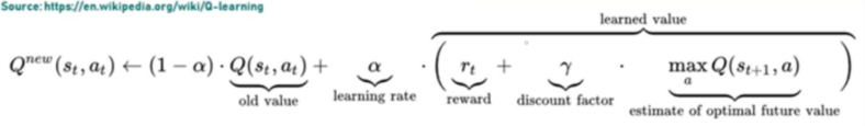
We then compute the new q-value and update the q-table using the below mentioned formula.

For the purpose of displaying the grid-world and the guys, we make an empty canvas, resize it as per the DISPLAY_SIZE parameter and paste the images of the agent, beer bottle and virus at their respective current locations.

At last we break the loop either if the agent gets his beer or if he gets infected by the virus.

We calculate the moving average and plot the rewards.

Finally we save the updated q-table.

Result

Following is the plot for the moving average of the rewards. It’s upward trend shows that the agent becomes smarter with more and more episodes of training.

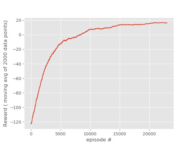Moving Average

And here are some GIFs that show how the agent gets smarter with every episode of training.

Here is the thirsty agent looking for the bottle of beer with randomly initialized q-table. It means that the agent has no clue about the environment yet.

dumb agent wants beer but does not get it

After some training, the agent does a relatively better job of making sequential decisions. He is not very fast yet but he ends up finding the beer eventually.

hmmm, that’s better

Finally after thousands of episode of training, the agent gets really good at making sequential decisions and finds the beer in no time ! : D

now that’s a smart-ass agent there ! B)

Advantages of Q-Learning

It is a simple concept to understand and implement. And it works great for environments with not a very huge state-action space.

Limitations of Q-Learning

Q-Learning involves look-ups from the q-table. And the q-table is made up of values for every single state-action pair possible. So as the state-space increases, the size of the q-table grows exponentially. So Q-Learning is good to train an agent in an environment with a small state-action space. For more complex set-ups , Deep Q-Learning is used.

Code

You can find the code for this q-learning project on my GitHub account by clicking on this link https://github.com/n0obcoder/Q-Learning

References

I am writing this blog because I have learned a lot by reading other’s blogs and I feel that I should also write and share my learnings and knowledge, as much as I can. So please leave your feedbacks in the comments section below to let me know how can I improve my future blogs ! :D

Share on

Twitter Facebook Google+ LinkedIn

Josue Ortega Caro, PhD